Backtracking strategy

 

Anytime you have a problem that is solved by a series of decisions there are chances that you might make a wrong decision and when you realize that you have to backtrack to a place where you made that decision and try something else, that what backtracking is. It is an efficient technique that uses a brute force approach to solve algorithm problems. In backtracking, we search depth-first for solutions backtracking to the last valid path as soon as we hit a dead end.

Backtracking decreases the search space since we at this point don’t need to follow down anyways, we know are invalid. This is called pruning. We should have the option to test a partial solution: for instance, we can’t track down global optimum utilizing backtracking, since we have no clue if the solution, we’re as of now on can prompt it or not. However, we can, for instance, address Sudoku utilizing backtracking. We can know quickly if our answer so far is invalid by testing if two of a similar number show up in a row, column, or square.

It is helpful to execute a backtracking algorithm by building a tree of decisions being made, called the state-space tree. Its root addresses an underlying state before the quest for an answer starts. The nodes of the primary level in the tree address the decisions made for the main segment of an answer, the nodes of the subsequent level address the decisions for the subsequent part, etc. A node in a state-space tree is supposed to be promising in the event that it relates to a somewhat constructed solution that may, in any case, prompt a final solution; else, it is called nonpromising.

Leaves address either nonpromising dead ends or final solutions found by the calculation. In most cases, a state-space tree for backtracking algorithm is developed in the way of depth-first search. In the event that the current node is promising, its child node is generated by adding the principal remaining choices for the following components of the solution, and the preparing moves to this child node. In the event that the current node ends up being nonpromising, the algorithm backtracks to the node’s parent to think about the following conceivable alternative for its last part; if there is no such choice, it backtracks one more level up the tree and so on. At last, if the algorithm arrives at the final solution for the question, it either stops (if only one is required) or keeps looking for other potential solutions.

There are three types of backtracking problems:

• Decision Problem — In this, we search for a feasible solution.
• Optimization Problem — In this, we search for the best solution.
• Enumeration Problem — In this, we find all feasible solutions.

Backtracking can be used in the problems that have clear and very much characterized requirements on any objective solution, that gradually assembles candidate to the solution and forsakes a candidate (“backtracks”) when it confirms that the candidate can’t in any way be finished to a substantial solution. Then again, backtracking isn’t viewed as a streamlined procedure to tackle a problem. It discovers its application when the solution required for an issue isn’t time-limited.

Consider a circumstance that you have three oranges before you and just one of them has a delicious taste however you don’t know which one. Thus, to get that delicious orange, you should peel off every orange individually. You will initially taste the primary orange, on the off chance that it doesn’t taste good, you should leave it as it is and peel the subsequent orange and so on until you find that delicious orange. This is the thing that backtracking is, that is tackling all sub-problems individually to arrive at the most ideal solution.

Consider the beneath instance to comprehend the Backtracking approach,

Given an example of any problem, P1 and data given as D1 comparing to the occasion, every one of the constraints that should be fulfilled to tackle the problem are addressed by C1. A backtracking algorithm will at that point function as follows:

The Algorithm starts to develop an answer, beginning with an unfilled solution set s. s = {}

1. Add to s the starting move that is still left (All potential moves are added to s individually). This presently makes another sub-tree st in the search tree of the algorithm.

2. Check if s+st fulfills every one of the constraints in C1.

On the off chance that Yes, the sub-tree st is “qualified” to add more “children”.

Else, the whole sub-tree st is pointless, so repeats back to stage 1 utilizing argument s.

3. In case of “qualification” of the recently shaped sub-tree st, repeats back to stage 1, utilizing contention s+st.

4. On the off chance that the check for s+st returns that it is an answer for the whole data D1. Output and end the program.

Assuming not, return that no solution is feasible with the current st and then delete it.

Backtracking is most often associated with recursion but the way backtracking happens with the recursive solution is tough to see and makes it difficult to write recursive backtracking solutions.

In recursion, the function calls itself until it arrives at a base case. In backtracking, we use recursion to investigate every one of the prospects until we get the best outcome for the problem.

Few popular problems related to backtracking algorithm are as follows:

• Hamiltonian cycle
• N-Queens problem
• Solving cryptarithmetic puzzles
• The knight’s tour problem
• Rat in a Maze
• m coloring problem
• Magnet Puzzle
• Flight itinerary problem

• The knight’s tour problem

Backtracking is used when we need to check all the possibilities to find a solution and hence it is expensive. For the problems like N-Queen and Knight's tour, there are approaches which take lesser time than backtracking, but for a small size input like 4x4 chessboard, we can ignore the running time and the backtracking leads us to the solution.

Knight's tour is a problem in which we are provided with a NxN chessboard and a knight.

For a person who is not familiar with chess, the knight moves two squares horizontally and one square vertically, or two squares vertically and one square horizontally as shown in the picture given below.

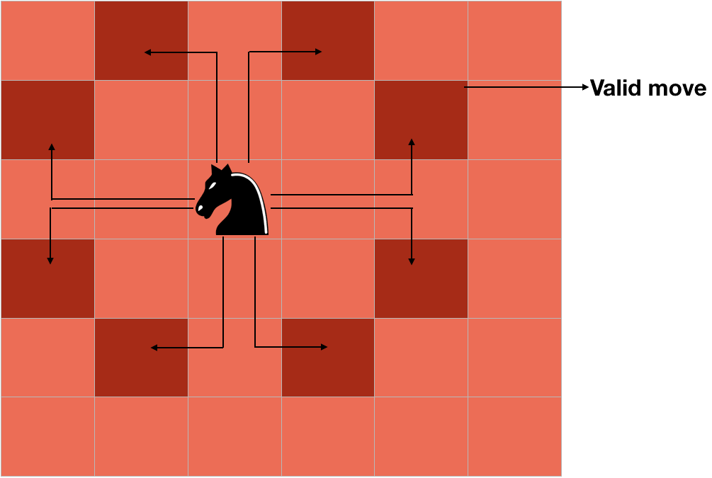
Thus if a knight is at (3, 3), it can move to the (1, 2) ,(1, 4), (2, 1), (4, 1), (5, 2), (5, 4), (2, 5) and (4, 5) cells.

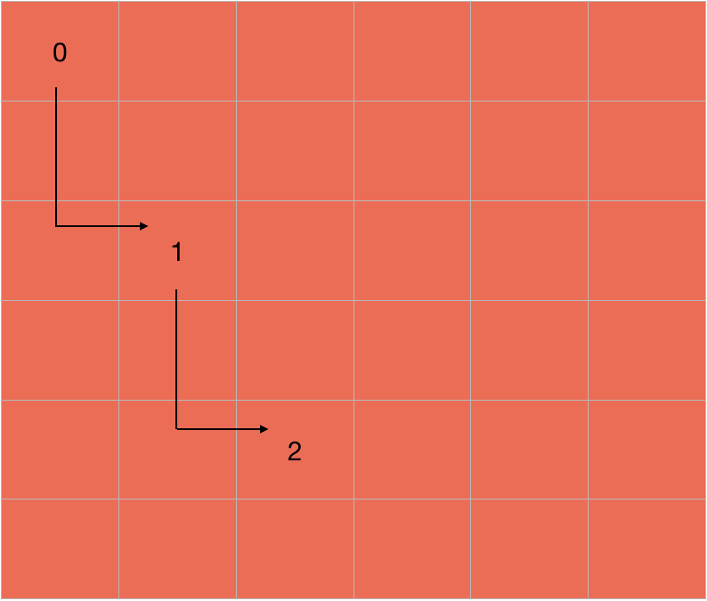
Thus, one complete movement of a knight looks like the letter "L", which is 2 cells long.

According to the problem, we have to make the knight cover all the cells of the board and it can move to a cell only once.

There can be two ways of finishing the knight move - the first in which the knight is one knight's move away from the cell from where it began, so it can go to the position from where it started and form a loop, this is called closed tour; the second in which the knight finishes anywhere else, this is called open tour.

Approach to Knight's Tour Problem

---

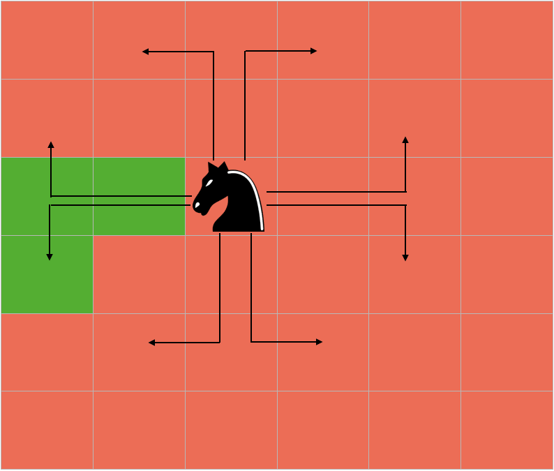
Similar to the N-Queens problem, we start by moving the knight and if the knight reaches to a cell from where there is no further cell available to move and we have not reached to the solution yet (not all cells are covered), then we backtrack and change our decision and choose a different path.

So from a cell, we choose a move of the knight from all the moves available, and then recursively check if this will lead us to the solution or not. If not, then we choose a different path.

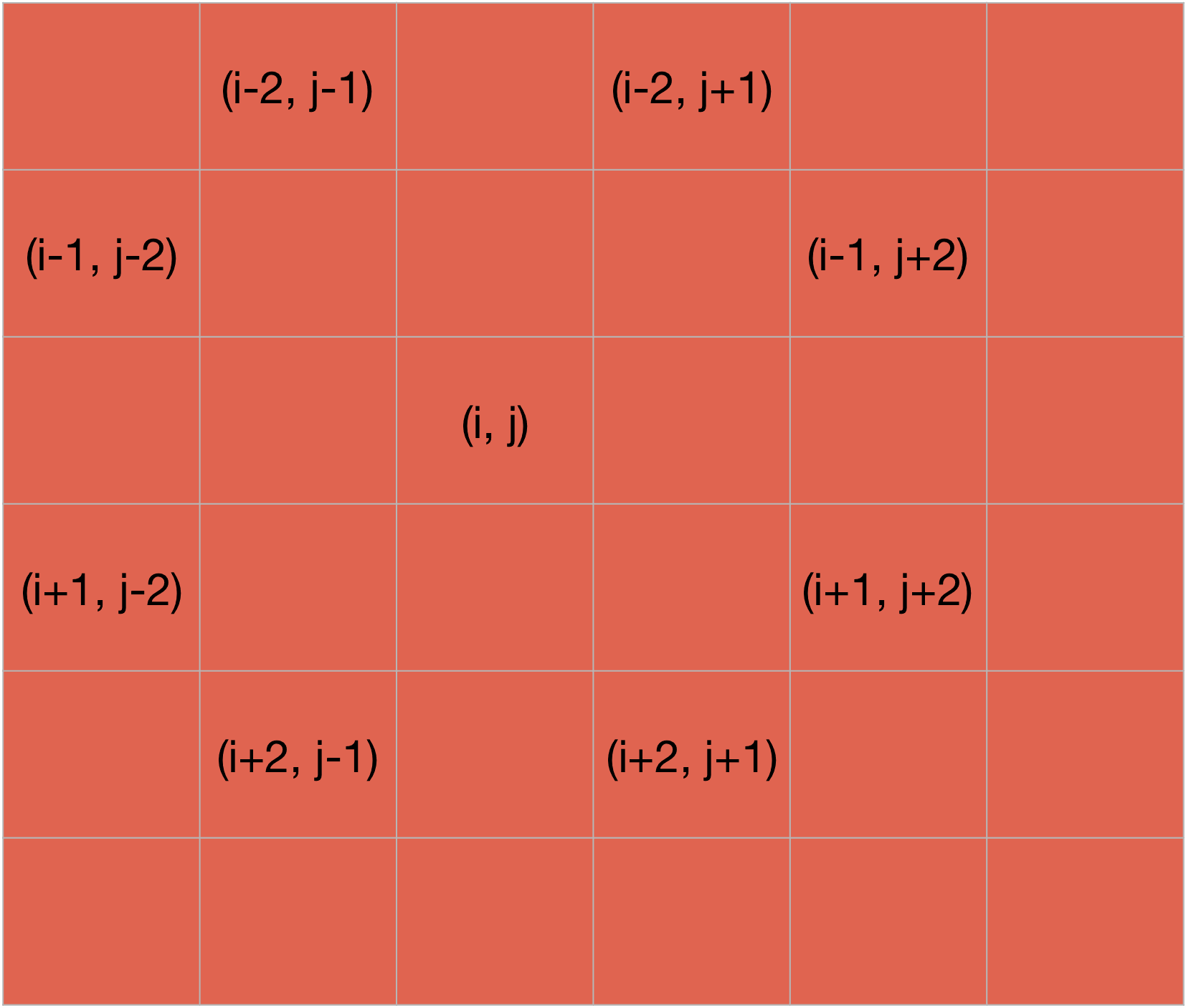
As you can see from the picture above, there is a maximum of 8 different moves which a knight can take from a cell. So if a knight is at the cell (i, j), then the moves it can take are - (i+2, j+1), (i+1, j+2), (i-2,j+1), (i-1, j+2), (i-1, j-2), (i-2, j-1), (i+1, j-2) and (i+2, j-1).

We keep the track of the moves in a matrix. This matrix stores the step number in which we visited a cell. For example, if we visit a cell in the second step, it will have a value of 2.

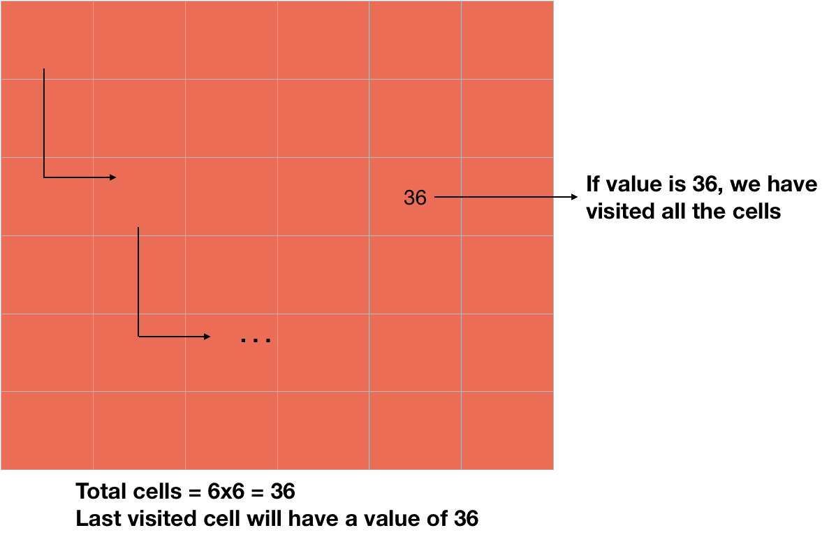
This matrix also helps us to know whether we have covered all the cells or not. If the last visited cell has a value of N*N, it means we have covered all the cells.

Thus, our approach includes starting from a cell and then choosing a move from all the available moves. Then we check if this move will lead us to the solution or not. If not, we choose a different move. Also, we store all the steps in which we are moving in a matrix.

Now, we know the basic approach we are going to follow. So, let's develop the code for the same.

Code for Knight's Tour

---

Let's start by making a function to check if a move to the cell (i, j) is valid or not - IS-VALID(i, j, sol). As mentioned above, 'sol' is the matrix in which we are storing the steps we have taken.

A move is valid if it is inside the chessboard (i.e., i and j are between 1 to N) and if the cell is not already occupied (i.e., sol[i][j] == -1). We will make the value of all the unoccupied cells equal to -1.

IS-VALID(i, j, sol)
  if (i>=1 and i<=N and j>=1 and j<=N and sol[i][j]==-1)
    return TRUE
  return FALSE

As stated above, there is a maximum of 8 possible moves from a cell (i, j). Thus, we will make 2 arrays so that we can use them to check for the possible moves.

x_move = [2, 1, -1, -2, -2, -1, 1, 2]
y_move = [1, 2, 2, 1, -1, -2, -2, -1]

Thus if we are on a cell (i, j), we can iterate over these arrays to find the possible move i.e., (i+2, j+1), (i+1, j+2), etc.

Now, we will make a function to find the solution. This function will take the solution matrix, the cell where currently the knight is (initially, it will be at (1, 1)), the step count of that cell and the two arrays for the move as mentioned above - KNIGHT-TOUR(sol, i, j, step_count, x_move, y_move).

We will start by checking if the solution is found. If the solution is found (step_count == N*N), then we will just return true.

KNIGHT-TOUR(sol, i, j, step_count, x_move, y_move)
  if step_count == N*N
    return TRUE

Our next task is to move to the next possible knight's move and check if this will lead us to the solution. If not, then we will select the different move and if none of the moves are leading us to the solution, then we will return false.

As mentioned above, to find the possible moves, we will iterate over the x_move and the y_move arrays.

KNIGHT-TOUR(sol, i, j, step_count, x_move, y_move)
  ...
  for k in 1 to 8
    next_i = i+x_move[k]
    next_j = j+y_move[k]

Now, we have to check if the cell (i+x_move[k], j+y_move[k]) is valid or not. If it is valid then we will move to that cell - sol[i+x_move[k]][j+y_move[k]] = step_count and check if this path is leading us to the solution ot not - if KNIGHT-TOUR(sol, i+x_move[k], j+y_move[k], step_count+1, x_move, y_move).

KNIGHT-TOUR(sol, i, j, step_count, x_move, y_move)
  ...
  for k in 1 to 8
    ...
    if IS-VALID(i+x_move[k], j+y_move[k])
      sol[i+x_move[k]][j+y_move[k]] = step_count
      if KNIGHT-TOUR(sol, i+x_move[k], j+y_move[k], step_count+1, x_move, y_move)
        return TRUE

If the move (i+x_move[k], j+y_move[k]) is leading us to the solution - if KNIGHT-TOUR(sol, i+x_move[k], j+y_move[k], step_count+1, x_move, y_move), then we are returning true.

If this move is not leading us to the solution, then we will choose a different move (loop will iterate to a different move). Also, we will again make the cell (i+x_move[k], j+y_move[k]) of solution matrix -1 as we have checked this path and it is not leading us to the solution, so leave it and thus it is backtracking.

KNIGHT-TOUR(sol, i, j, step_count, x_move, y_move)
  ...
  for k in 1 to 8
    ...
      sol[i+x_move[k], j+y_move[k]] = -1

At last, if none the possible move returns us false, then we will just return false.

KNIGHT-TOUR(sol, i, j, step_count, x_move, y_move)
  if step_count == N*N
    return TRUE

  for k in 1 to 8
    next_i = i+x_move[k]
    next_j = j+y_move[k]
    if IS-VALID(next_i, next_j, sol)
      sol[next_i][next_j] = step_count
      if KNIGHT-TOUR(sol, next_i, next_j, step_count+1, x_move, y_move)
        return TRUE
      sol[next_i, next_j] = -1

  return FALSE

We have to start the KNIGHT-TOUR function by passing the solution, x_move and y_move matrices. So, let's do this.

As stated earlier, we will initialize the solution matrix by making all its element -1.

for i in 1 to N
  for j in 1 to N
    sol[i][j] = -1

The next task is to make x_move and y_move arrays.

x_move = [2, 1, -1, -2, -2, -1, 1, 2]
y_move = [1, 2, 2, 1, -1, -2, -2, -1]

We will start the tour of the knight from the cell (1, 1) as its first step. So, we will make the value of the cell(1, 1) 0 and then call KNIGHT-TOUR(sol, 1, 1, 1, x_move, y_move).

START-KNIGHT-TOUR()
  sol =[][]
  for i in 1 to N
    for j in 1 to N
      sol[i][j] = -1

  x_move = [2, 1, -1, -2, -2, -1, 1, 2]
  y_move = [1, 2, 2, 1, -1, -2, -2, -1]

  sol[1, 1] = 0

  if KNIGHT-TOUR(sol, 1, 1, 1, x_move, y_move)
    return TRUE
  return FALSE

RAT IN A MAZE

Rat in a maze is also one popular problem that utilizes backtracking. If you want to brush up your concepts of backtracking, then you can read this post here. You can also see this post related to solving a Sudoku using backtracking.

A maze is a 2D matrix in which some cells are blocked. One of the cells is the source cell, from where we have to start. And another one of them is the destination, where we have to reach. We have to find a path from the source to the destination without moving into any of the blocked cells. A picture of an unsolved maze is shown below.

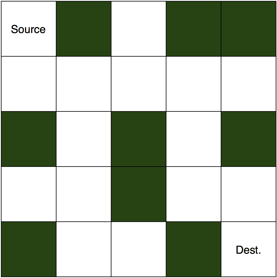
And this is its solution.

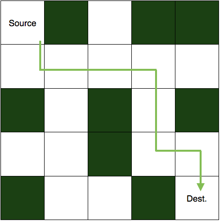
To solve this puzzle, we first start with the source cell and move in a direction where the path is not blocked. If taken path makes us reach to the destination then the puzzle is solved else, we come back and change our direction of the path taken. We are going to implement the same logic in our code also. So, let's see how.

Algorithm to solve a rat in a maze

---

You know about the problem, so let's see how we are going to solve it. Firstly, we will make a matrix to represent the maze, and the elements of the matrix will be either 0 or 1. 1 will represent the blocked cell and 0 will represent the cells in which we can move. The matrix for the maze shown above is:

0 1 0 1 1

0 0 0 0 0

1 0 1 0 1

0 0 1 0 0

1 0 0 1 0

Now, we will make one more matrix of the same dimension to store the solution. Its elements will also be either 0 or 1. 1 will represent the cells in our path and rest of the cells will be 0. The matrix representing the solution is:

1 0 0 0 0

1 1 1 1 0

0 0 0 1 0

0 0 0 1 1

0 0 0 0 1

Thus, we now have our matrices. Next, we will find a path from the source cell to the destination cell and the steps we will take are:

1. Check for the current cell, if it is the destination cell, then the puzzle is solved.
2. If not, then we will try to move downward and see if we can move in the downward cell or not (to move in a cell it must be vacant and not already present in the path).
3. If we can move there, then we will continue with the path taken to the next downward cell.
4. If not, we will try to move to the rightward cell. And if it is blocked or taken, we will move upward.
5. Similarly, if we can't move up as well, we will simply move to the left cell.
6. If none of the four moves (down, right, up, or left) are possible, we will simply move back and change our current path (backtracking).

Thus, the summary is that we try to move to the other cell (down, right, up, and left) from the current cell and if no movement is possible, then just come back and change the direction of the path to another cell.

N-QUEEN PROBLEM

In the N-Queen problem, we are given an NxN chessboard and we need to put n queens on the board so that no two queens assault one another. A queen will assault another queen on the off chance that it is put in vertical, horizontal, or diagonal points in its direction.

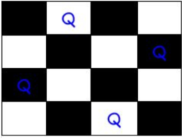
The binary output with 1’s as queens to the positions are placed:

{0 , 1 , 0 , 0}

{0 , 0 , 0 , 1}

{1 , 0 , 0 , 0}

{0 , 0 , 1 , 0}

we will take a stab at setting the queen into various positions of one row. What’s more, checks on the off chance that it conflicts with the different queen. In the event that current situating of queens if there are any two queens assaulting one another. On the off chance that they are assaulting, we will backtrack to the past location of the queen and change its positions. Furthermore, check the conflict of the queen once more.

ALGORITHM FOR N-QUEEN PROBLEM

CONCLUSION

Backtracking algorithm is regularly applied to troublesome combinatoric problems for which no effective algorithm for finding, precise solutions potentially exists. It creates all components of the problem state and takes care of each example of a problem in a satisfactory measure of time. Backtracking stays a legitimate and indispensable tool for taking care of different sorts of problems, despite the fact that this present algorithm’s time intricacy might be high, as it might have to investigate every single existing solution.